Robins 1986
During 2020, I read through Robins, J. (1986). “A new approach to causal inference in mortality studies with a sustained exposure period—application to control of the healthy worker survivor effect”. Mathematical modelling, 7(9-12), 1393-1512. This was all shared on Twitter. As I deleted my Twitter account long ago now, this thread disappeared along with it. To preserve it, I now host it here.
Below is all from the original 2020 thread. There is likely different elements I would emphasize now, but I leave that for a future date.
Setup
Because I have been meaning to read through it fully and this is a better way to keep myself accountable, a thread as I (we) read through Robins 1986. (Also writing it out helps me think better)
I will probably do a section every (or every few) day(s) Some of my nomenclature:
- CI – Causal inference
- RR – Risk Ratio
- HWE – Healthy worker effect
- DAG - Directed Acyclic Graph
- LTFU - lost-to-follow-up
- RCT - randomized control trial (overlook the ‘control’ in some of the discussion, I use for ease of abbrev.)
(going to regret not putting more here)
1: INTRODUCTION
After 3 pages of vocab and the section it is defined in, we start with the introduction.
Robins begins with the difficulty of defining an appropriate comparison for a working population, since an unexposed* working pop is ‘healthier’ than the general pop

I think most importantly is that Robins sets out to identify ‘small’ effects since most large occupational exposures already have been discovered. I think this stands in stark contrast to claims about CI being less appropriate for small effects or sensitivity analyses (E-values).
To avoid the HWE, workers with different levels of exposure are compared. However, the standard methods of looking at cumulative exposures can mask those small effects Robins is interested in.

To relate to the larger literature, he mentions this paper by Gilbert. This approach is later said to be commonly used in occupational epi (at the time).
Gilbert 1982 talks about occupational factors at the Hanford nuclear site on mortality. Gilbert says that differences in mortality between employed and terminated works are sources of bias due to the healthy worker effect.


To address this, workers were considered as ‘employed’ up to 3 years after their termination. Gilbert’s approach works as a sort of ‘wash-out’ period for occupational exposures. However, Robins says this wash-out approach doesn’t work and we will see this in occupational exposure to arsenic. He gives us a teaser (so we get through the following 100+ pages).
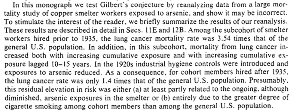
Occupational arsenic has been decreased post-1935 but lung cancer has remained elevated among copper smelter workers. This could be due to (1) remaining arsenic exposures, or (2) elevated cigarette smoking among workers. Using the lagging approach, cumulative exposure to arsenic has no association with lung cancer mortality. However, Robins’ proposed approach does find elevated lung cancer mortality. He conjectures that it is due to smokers leaving employment more than non-smokers. He can’t directly tell us (so a bit of a letdown).
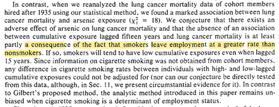
Robins then says that using the proposed method is necessary because of reduced occupational exposures leading to smaller effects (as indicated by RR).
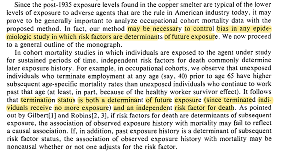
Then he hit us with the succinct purpose of the paper; when do we get to give causal interpretations for time-varying exposures with observational data. Robins then outlines what each section will discuss. I won’t repeat / spoil it though (but it would be great to do a SPOILER ALERT for a paper that is older than me).
2: OBS STUDY AS RCT
This section is probably one of the most important insights, framing observational data as a randomized trial conducted by nature (I think I might like causal inference as a missing data problem more though).
We start with an example. To add, I am going to adapt a quick example to illustrate his previous point regarding ‘small effects’ from Section 1 to highlight the importance of his previous argument. Pictured is a DAG for a data generating mechanism and some Python code.
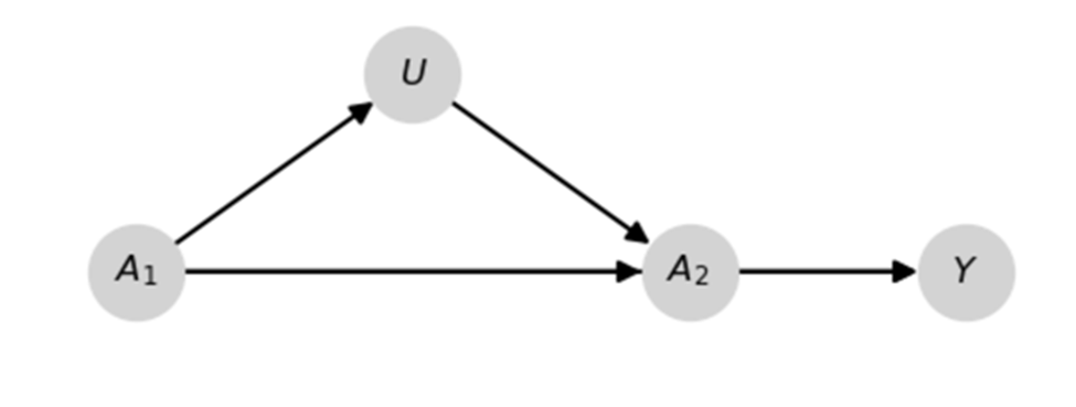
import numpy as np
import pandas as pd
import matplotlib.pyplot as plt
from zepid.causal.causalgraph import DirectedAcyclicGraph

# Drawing a DAG
dag = DirectedAcyclicGraph(exposure=r"$$A_1$$", outcome=r"$Y$")
dag.add_arrows(((r"$A_1$", r"$Y$"),
                (r"$A_2$", r"$Y$"),
                (r"$A_1$", r"$A_2$"),
                (r"$A_1$", r"$U$"),
                (r"$U$", r"$A_2$")))
dag.draw_dag(fig_size=(6, 4),
             positions={r"$A_1": (1, 1),
                        r"$A_2": (3, 1),
                        r"$U": (2, 1.05),
                        r"$Y": (4, 1)})
plt.show()

# Generating data
np.random.seed(1986)
n = 1000000

# Defining potential outcomes
df = pd.DataFrame()
df['y_a0a0'] = np.random.binomial(n=1, p=0.4, size=n)
df['y_a1a0'] = np.random.binomial(n=1, p=0.45, size=n)
df['y_a0a1'] = np.random.binomial(n=1, p=0.55, size=n)
df['y_a1a1'] = np.random.binomial(n=1, p=0.6, size=n)

# Alloting treatments
df['A_1'] = np.random.binomial(n=1, p=0.5, size=n)
df['U'] = np.random.binomial(n=1, p=0.2 + 0.4*df['A_1'], size=n)
df['A_2'] = np.random.binomial(n=1, p=df['A_1']*0.85 +
                                      (1-df['A_1'])*0.15 -
                                       0.1*df['U'], size=n)

# Applying causal consistency
df['Y'] = (df['A_1']*df['A_2']*df['y_a1a1'] +
           (1-df['A_1'])*df['A_2']*df['y_a0a1'] +
           df['A_1']*(1-df['A_2'])*df['y_a1a0'] +
           (1-df['A_1'])*(1-df['A_2'])*df['y_a0a0'])
Since $A$ is randomized at baseline ($t_1$), we can easily estimate $\Pr(Y(a_1))$ with $\Pr(Y \mid A_1=a_1)$ where $Y(a_1)$ is the potential outcome under $a_1$. In my example $\hat{\Pr}(Y \mid A_1=1) / \hat{\Pr}(Y \mid A_1=0)$ is
# Calculating Risk Ratio
from zepid import RiskRatio

rr_est = RiskRatio()
rr_est.fit(df, exposure='A_1', outcome='Y')
rr_est.summary()

# RiskRatio  SD(RR)  RR_LCL  RR_UCL
#     1.354   0.002   1.349    1.36
However, I am using 1mil observations for that estimate. That’s probably more than we have in most scenarios. Under the more realistic case of 750 observations, things are less clear.
rr_est = RiskRatio()
rr_est.fit(df.sample(n=750), exposure='A_1', outcome='Y')
rr_est.summary()

# RiskRatio  SD(RR)  RR_LCL  RR_UCL
#     1.172   0.074   1.014   1.355
Since we are using some simulated data, we can check another estimand $\Pr(Y(a_1, a_2))$. For cumulative effects (i.e., effect is monotonic over time), $\Pr(Y(a_1, a_2)) \ge \Pr(Y(a_1))$. This means we have a better chance of identifying ‘small effects’ of $A$ by targeting $\Pr(Y(a_1, a_2))$.
# Calculating Pr(Y(a_1, a_2)_ directly
print(np.mean(df['y_a1a1']) / np.mean(df['y_a0a0']))
# RiskRatio
#     1.502
However, using $\Pr(Y \mid A_1=a_1, A_2=a_2))$ doesn’t correctly estimate the previous quantity because of the $U$ I drew in the previous DAG. That’s why we need this paper and the proposed method.
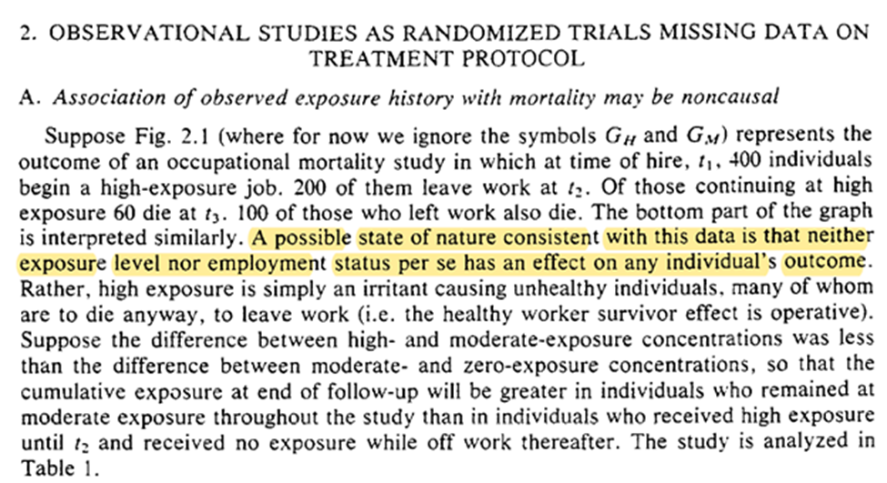
Already we are given a glimpse of what Robins is talking about when he talks about using time-varying exposures to identify effects. Returning to Robins example, he gives us this nice tree ($G_m$ is moderate exposure)
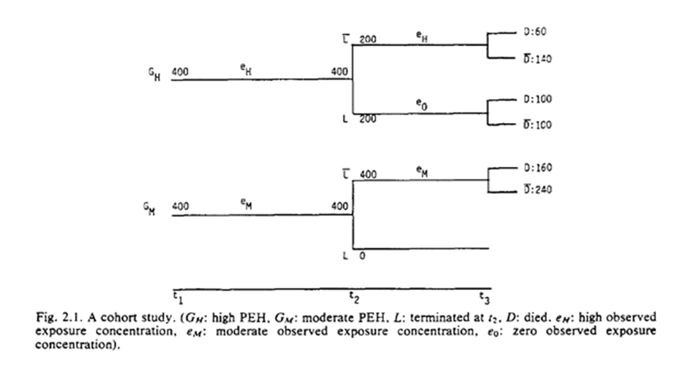
He gives us a table based on some categorizations of the exposures (I have an updated table below). As seen, high exposure seems protective. However, we know this isn’t true (the exposure has no effect).
| High | Moderate | Low | |
|---|---|---|---|
| Events | 60 | 160 | 100 |
| Total | 200 | 400 | 200 |
| Risk | 0.3 | 0.4 | 0.5 |
| Risk Ratio | 0.6 | 0.8 | 1 |
Rather it is a result of the exposure being an irritant and resulting in unhealthy individuals quitting work earlier than healthy individuals.
Robins mentions in this section, if we had treated the baseline assignment of exposure categories (high vs medium) at $t_1$, we would correctly have estimated no effect: $RR = (160/400) / (160/400) = 1.0$
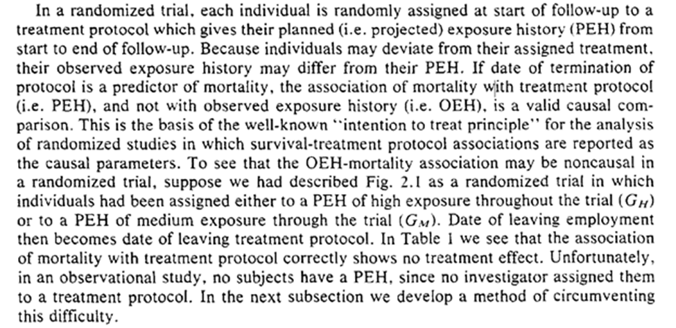
We see how to foundation of observational studies as a randomized trial. Our collaborator, Dr. Nature, isn’t always the most organized and seemingly forgets to forward the randomization protocol to us. A primary challenge is determining when we consider an individual to deviate from their assigned protocol.
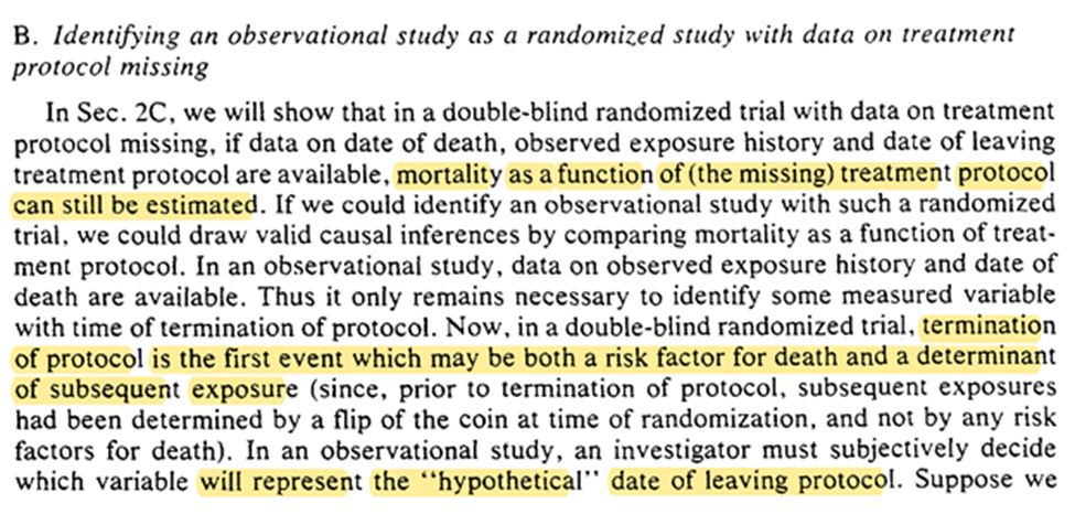

Robins states if we (accurately) measure day of death, exposure history, date of leaving the exposure protocol, then we can estimate mortality. The trick for translating obs. data into this is to determine when individuals leave the protocol.
A related issue (one-sample rather than the two-sample problem Robins is addressing) is when to consider someone as censored (LTFU). Lesko et al. have a nice discussion of when we should consider someone as censored.
For Robins’ example date of termination of employment works well as the time of deviation from protocol. He also tells us a similar exposure protocol end date for the mining industry.
The technical note simplifies the examples being discussed by simplifying the protocol. When we get to section 10, we will see how we can have more complex exposure plans (eg work every other year).
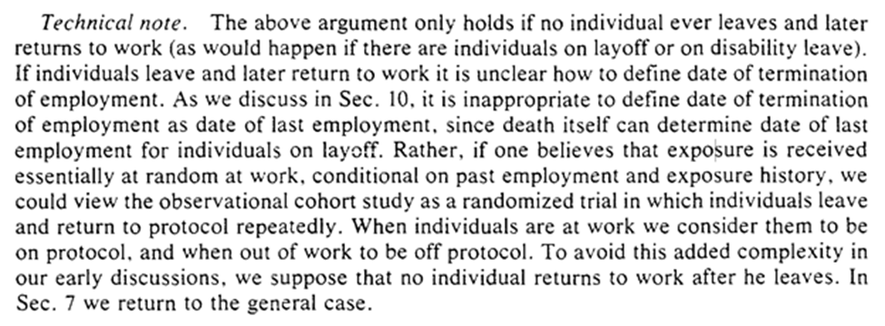
We get some notation: $G(t)$ is the projected exposure history and $E(t)$ is the observed exposure history. In other words $G(t)$ is the assigned RCT assigned protocol up to t and the $E(t)$ is the actual exposures.

2C.1 is treatment-variation-irrelevance, 2C.2 simplifies our problem (and we will relax it in section 10), 2C.3 removes more complex exposure plans that depend on measures at $t$.

The first sentence requires that the past exposure cannot be determined by future events (something we assume impossible about reality, but can accidentally do in analyses).

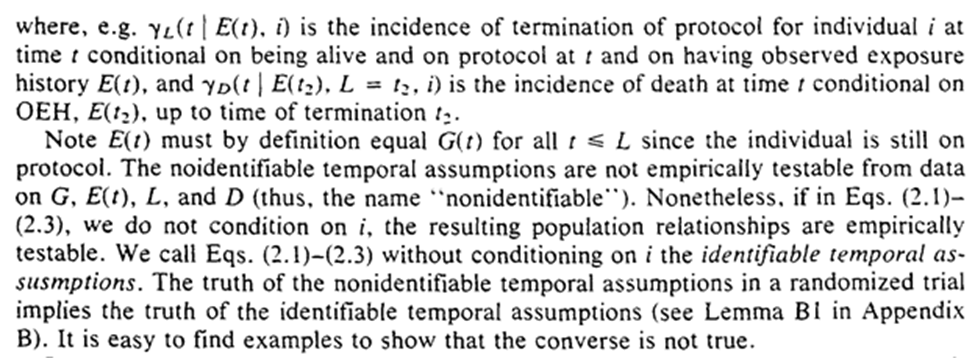
Imposing that time-order is for the 3 assumptions, which allows us to freely condition on $G$ (the projected exposure history). The individual-level assumptions imply the truth of the population-level versions.

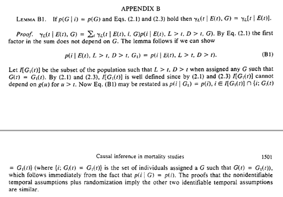
In our hypothetical trial on employment termination, the protocol cannot be influenced by unmeasured risk factors (randomization is used to make this true).
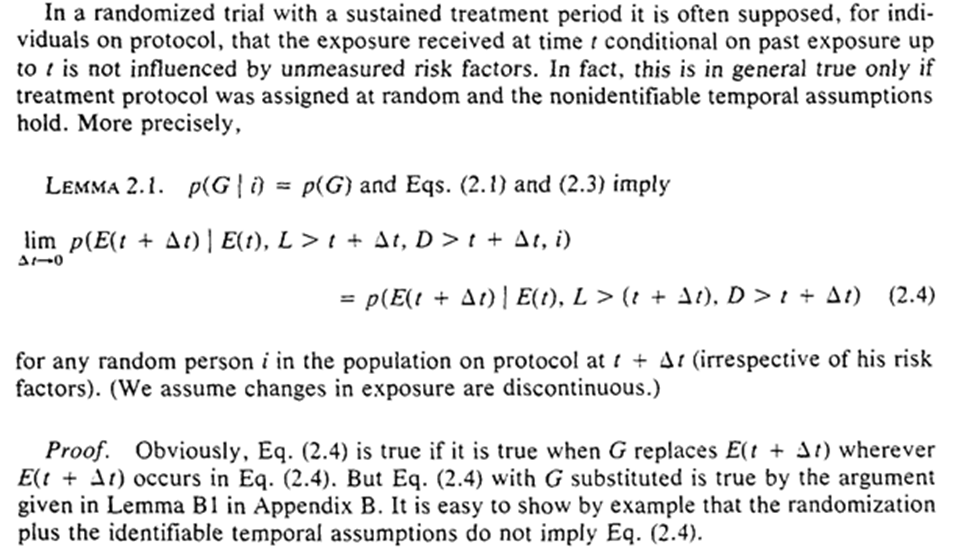
Under these conditions, we can consistently estimate survival without the actually assigned protocols! We only need the observed exposure history and when the protocol was terminated.

Robins gives a proof of this by showing the exclusive ways individual $i$ can survive to $t$ – survive on protocol to $t$, terminate protocol at $t-1$ and survive to $t$.
Interestingly, even if we did have information on the assigned protocol, it won’t provide any additional information. We could ignore it even if we had it.
This is only a cursory glance at his proofs (I need to work through them but the thread will be insanely long if I do here).
Now we can think about RCT where exposure is randomly assigned at t based only on previous exposure history. So we may no longer have a well-defined treatment plan at baseline.

This alt-RCT is a special case of the previous RCT! Specifically in which we don’t get to see the exposure protocol.
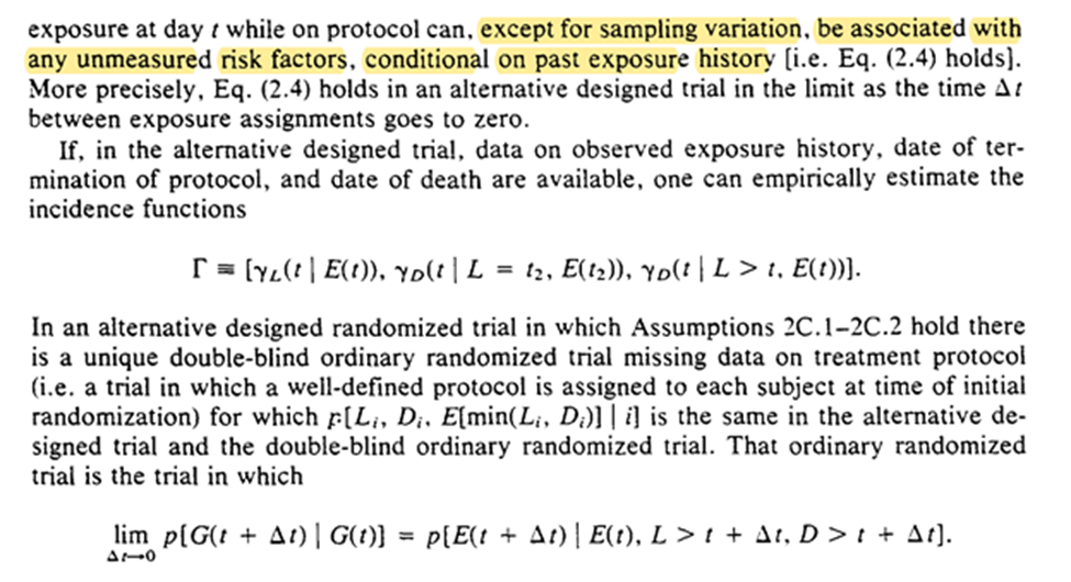
Robins concludes the section with mention that survival is a function of time and exposure can be beneficial / harmful at certain times (ie the stratified survival curves are allowed to cross).

We end this section with knowledge that we don’t need the exposure protocol to analyze our RCT. Now the question is when does obs. data reflect a RCT (or rather under what assumptions)
3: GRAPHS FOR CAUSAL INFERENCE
This section tells us the theoretical framework for when causality can be inferred from obs. data (under the FFR-CISTG model) We start with the process.
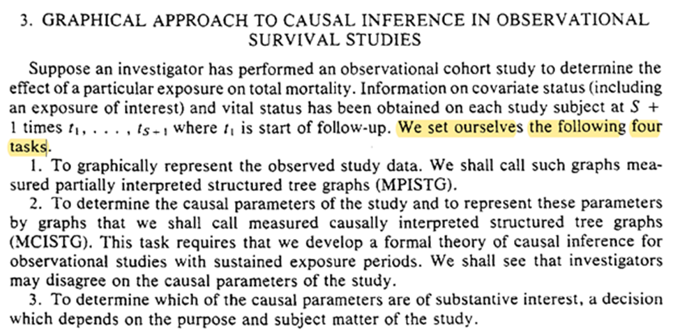

First, we draw a tree to represent the data we get to see (MPISTG)
Next, we define the causal parameters through a tree graph (MCISTG)
Next, we determine the causal parameters of interest
Lastly, we use an algorithm to estimate causal parameters from a final tree graph
Luckily for me, we start with informal descriptions. Here we are asked to consider two studies, much like the quick examples I wrote in Python in the previous section. We jump into drawing the tree graphs
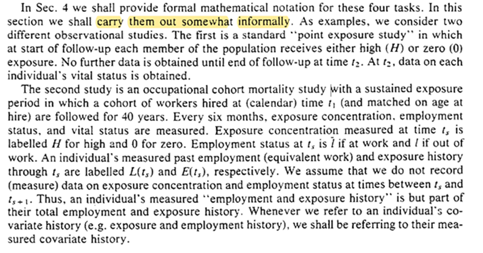
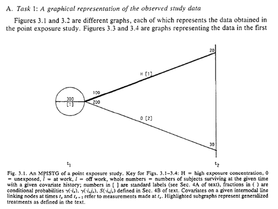
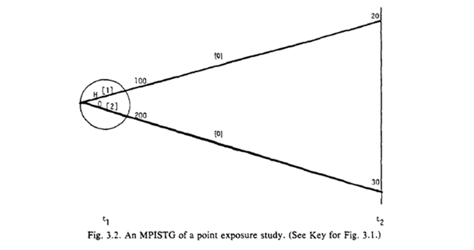
Fig 3.1-3.2 are STG for our point exposure study. Open circles are follow-up times (but omitted at final time), splits in the graph distinguish exposures at the circle. For 3.1 the population beings with 300 of which 100 are $A=1$. 20 survived until $t_2$.
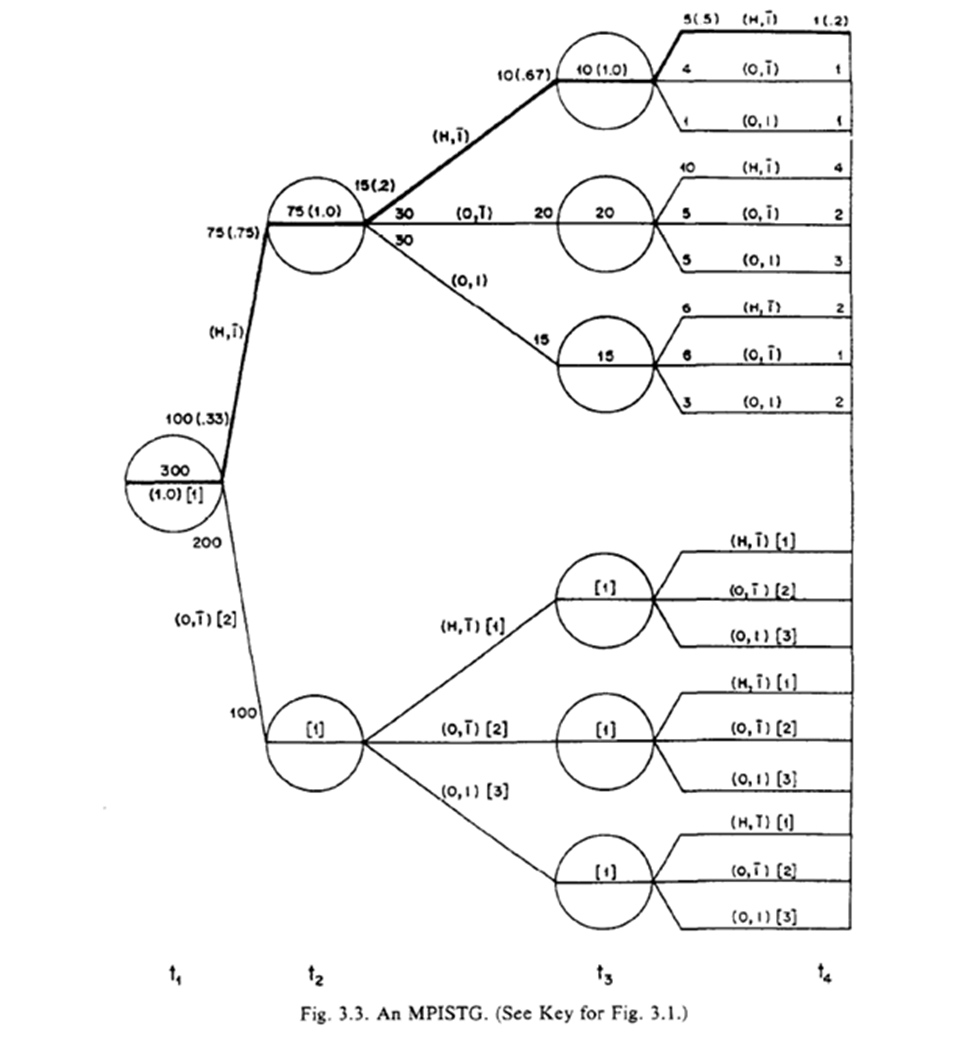
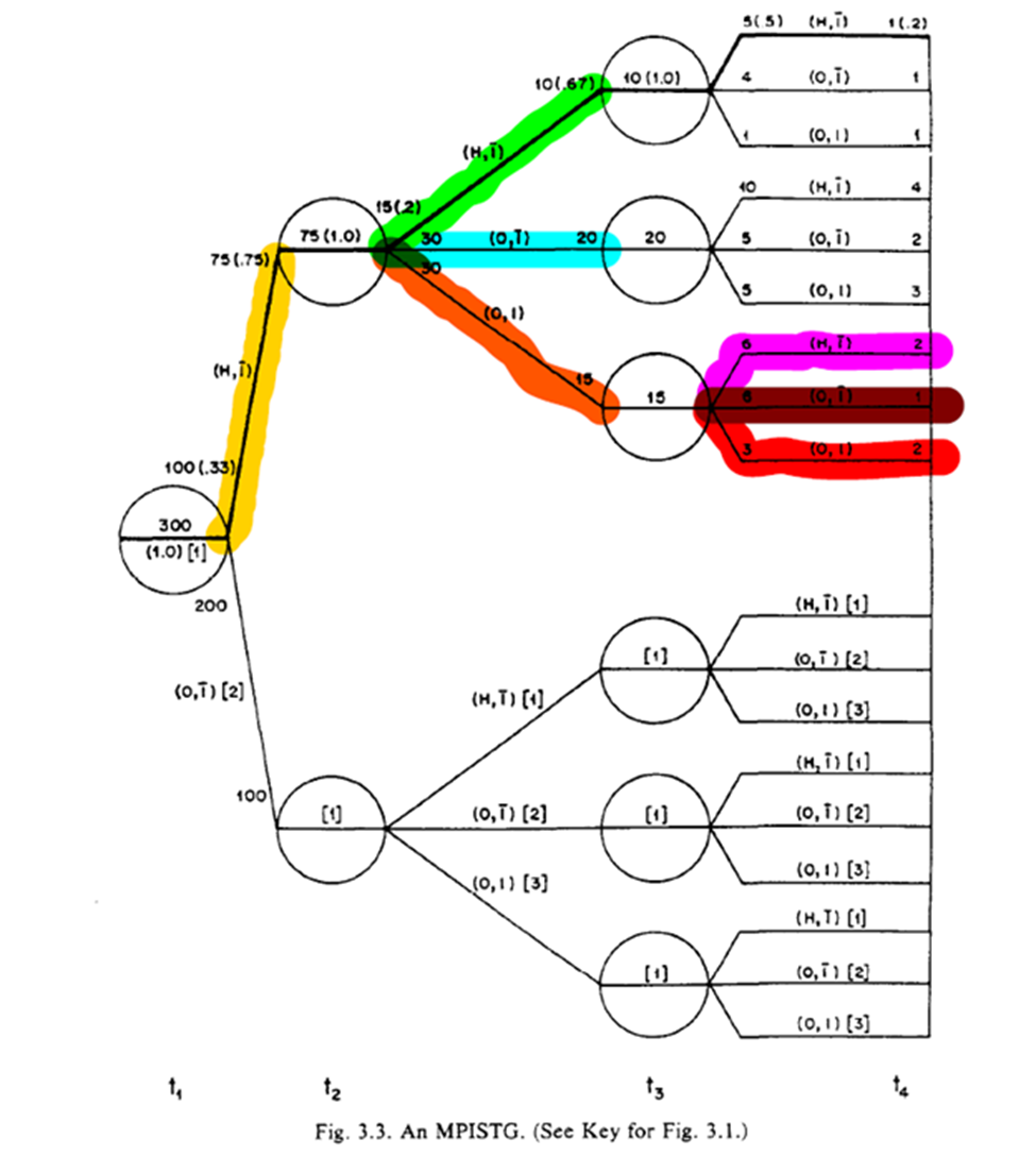
The STG in 3.3 follow a similar interpretation, but we also have more paths. Below is a highlight pattern of the figure to match the text descriptions. As shown, 4 periods of follow-up and only two variables still makes this complicated to draw
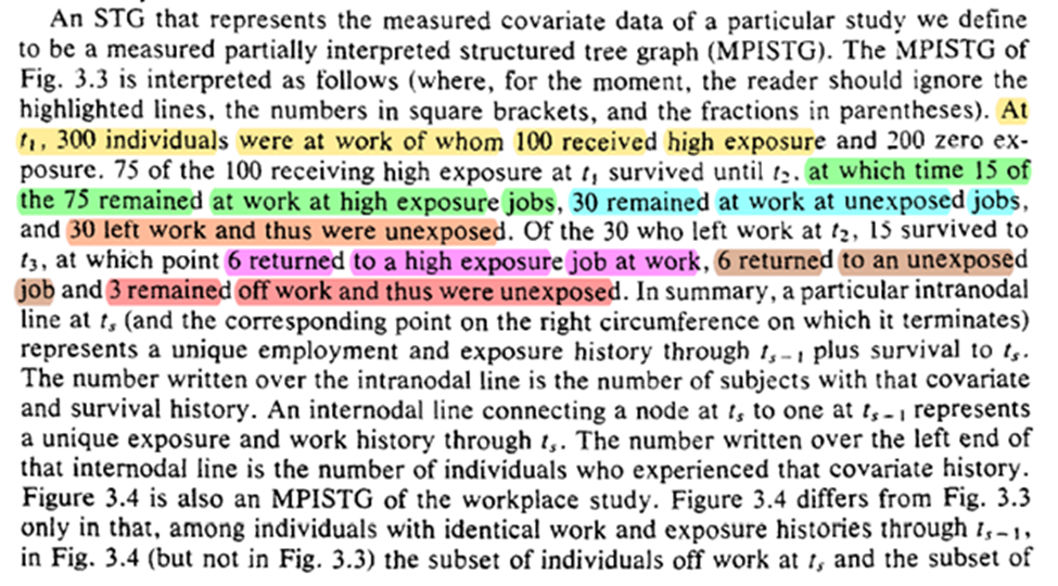
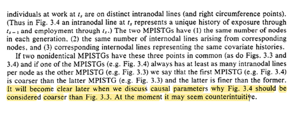
Robins goes on to distinguish between 3.3 and 3.4, with 3.4 being characterized as ‘finer’ as opposed to ‘coarse’. The difference is where the splits occur (something I missed when reading at first)
Honestly not sure I follow what the distinction really means … (Robins assures me that the discussion of causal parameters will make this clear)
With that, we are on to identifying the causal parameters of the study. We are extending Rubin’s framework to time-varying exposures. We do require the special case of deterministic potential outcomes at this point (not required by Rubin’s system)

This is fine for Rubin’s system since deterministic potential outcomes are a special case of stochastic potential outcomes (i.e. deterministic are a subset of stochastic)
We have 3 subtasks: define treatment, define the MCISTG, and the causal parameter of the study
Treatment is a variable that a particular individual could have been given/exposed to at time t. Robins says that treatment could have been randomized (at least in conception) is necessary for causal inference.
There is lots of discussion on this point, but I think it is worth highlighting since this is a major deviation between Pearl’s NPSEM and Robins’ FFR-CISTG. Especially since this distinction occurs before we have any discussion of mediation.
In the stairs example, we also get non-random (or structural) violations of the positivity assumption. This also demonstrates Robins’ previous point but I think restricting the population of interest is a solution to positivity but not always to causal consistency.

The non-existence of any non-random positivity violations is necessary to link the observed STG to the STG meant to define the causal parameters. I think about this as the observed data allows us to say something regarding a potential world.
On to the next subtask: defining the causal parameters
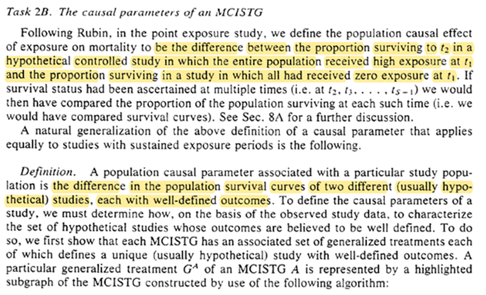
The algorithm to define treatments relies on lines splitting at the left-side (green) of the circle rather than the right-side (red). Where the line splits distinguish between the two highlighted statements (which answers my previous question)
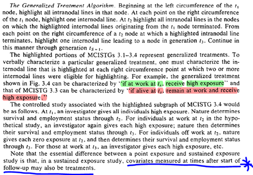
The final sentence is interesting to me, because we already have the concept of mediation being introduced. It highlights the link between time-varying exposures (that are the same exposure just at different times) and mediation
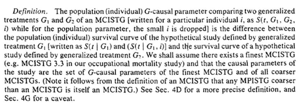
Finally we get our definition of what the causal parameter is. It is the difference between two proposed ‘generalized treatment plans’. I am going to try to keep the final parts in mind for when we get to section 4.
Task 3: decide what causal parameters we are actually interested in. Robins gives several examples (which I won’t repeat). I will highlight the last paragraph though.
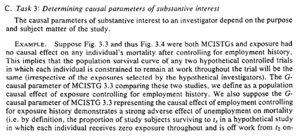
We end with a note on generalizability / transportability. Lesko et al. have a great paper on this as well

Finally, we determine what we can estimate given the observed data. Going back to ‘coarse’ we can estimate the MCISTG of any STG that is $\ge$ coarse for a valid generalized treatment plan
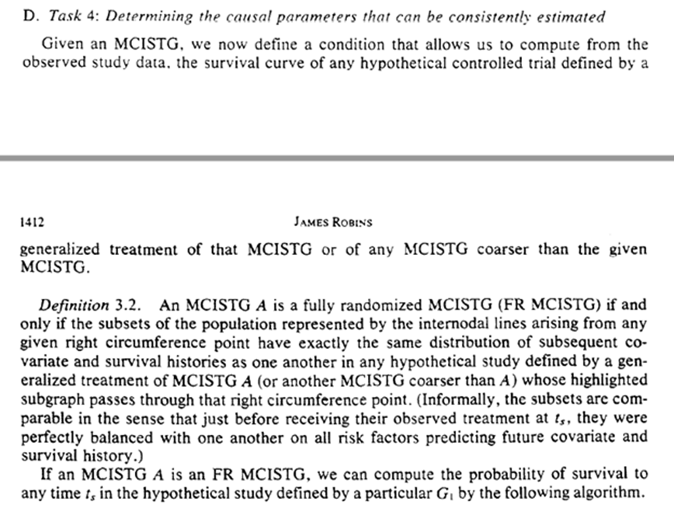
For the ‘fully randomized’ STG (FR-MCISTG) we need that there are no common causes (i.e. no confounding) of the exposure at t and the outcome. We now have how obs. data can be seen as a stratified RCT where Dr. Nature forgot to give us the stratification.
Now we get g-computation and how to do it! Calculate the conditional probabilities for survival then take the summation of these probabilities for the treatment plan of interest.
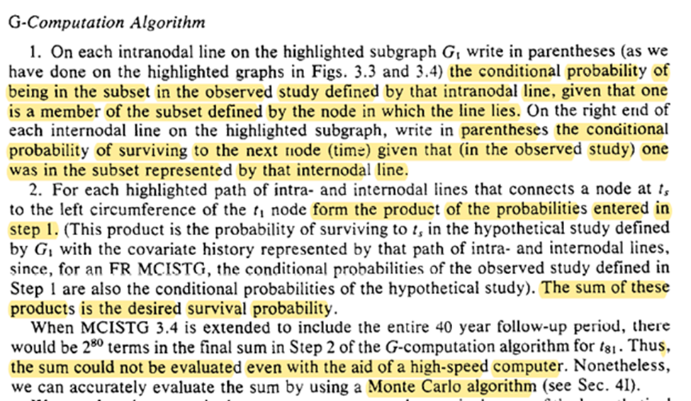
Easy! (See Snowden et al. 2011 for an easy algorithm for point-exposures). However, multiple time-points makes it difficult (if not impossible). Luckily we have a Monte Carlo extension (to be seen in section 4).
Unfortunately we can never ensure that our MCISTG is a FR-MCISTG. However saying we can’t possibly verify this ever doesn’t justify not conducting any observational studies Robins gives us a formal justification with regards to what we are assuming

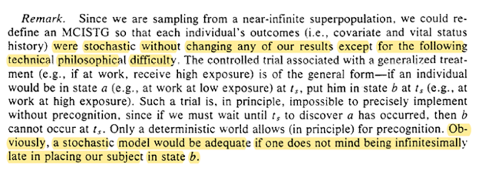
We also have a remark on whether we can apply FR-MCISTG to stochastic potential outcomes. We just have to ignore that our trial makes a slight mix-up wrt time (i.e. we either know something about the future or the randomization moves back in time).
I am going to skip over some practical points that Robins discusses in this thread (but you should read section 3D).
In 3E further discussion of the difference between 3.3 and 3.4. I am also going to leave this out for practical purposes. Briefly, we see further examples / problems of not being able to draw the observed STG with splits within the circles
At the end of s3F there is a brief tangent on a Bayesian view which isn’t adopted in this paper. Keil et al. 2017 have a good discussion of a Bayesian g-formula
Next time Robins gives us a formalization of section 3 (I have a feeling it will be a long thread)
4: FORMAL CAUSAL INFERENCE (ATTIRE REQUESTED)
Math on twitter dot com? Should be fine /s (ed: it is now with MathJax on the site). Shorter thread though
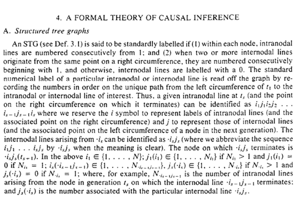
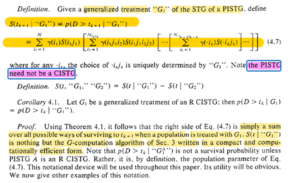
In Section 4.C we get a quirk of the deterministic results. Essentially within the deterministic system that nature created, the exposure pattern between $t_0$ and the end of the study has been ‘set’, no matter when outcomes occur. This is used to extend to competing risks.
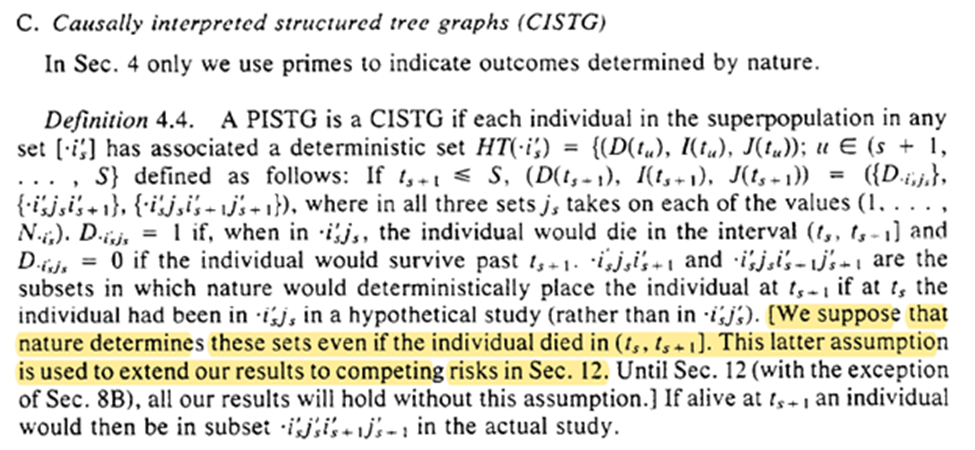
Here we get the written version of g-computation from Section 3. There is also the important point that g-comp can be applied to non-causal scenarios. However, when we do this there is less solid of interpretational foundations for the estimate
The assumptions are to link reality to the math formula. Without the assumptions about what happens in the world, the math is just a calculation exercise.
However, evaluating equation 4.7 is difficult for anything besides a small number of follow-up times. Robins proposes using Monte Carlo instead

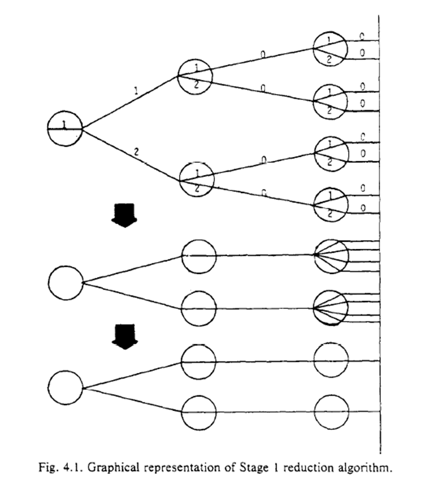
Robins concludes with an algorithm to reduce the complexity of the procedure. The procedure generates a coarser STG. While I don’t collapse the branches in my animation example, you can kinda see how non-time-varying exposures are a special case of a coarse STG
5: ESTIMATION
After a little hiatus, back to discussing Robins 1986 (with a new keyboard)! Robins starts by reminding us (me) that we are assuming the super-population model for inference.
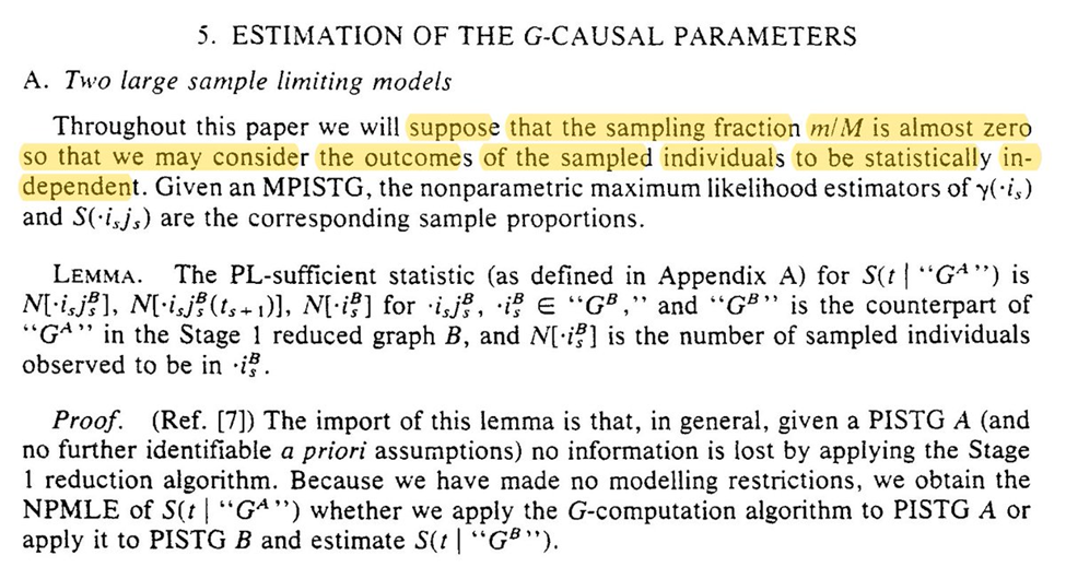
If we had an infinite $n$ in our study, we could use NPMLE. However, time-varying exposures have a particular large number of possible intervention plans. We probably don’t have anywhere near enough obs to consider all the possible plans
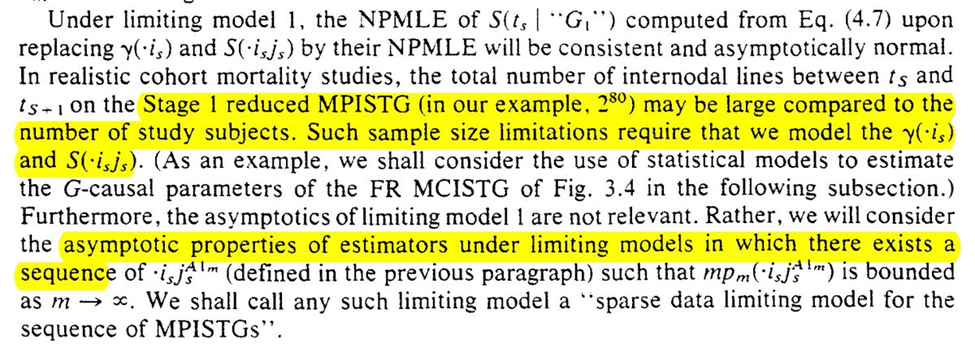
Instead we use a parametric projection of the time-varying variables. We hope that the parametric projection is sufficiently flexible to approximate the true density function (it is why it is best to include as many splines and interaction terms as feasible)
We now move to the arsenic example to connect the method discussed in the previous section
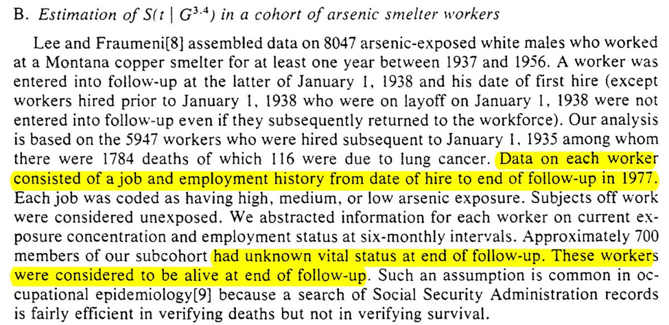
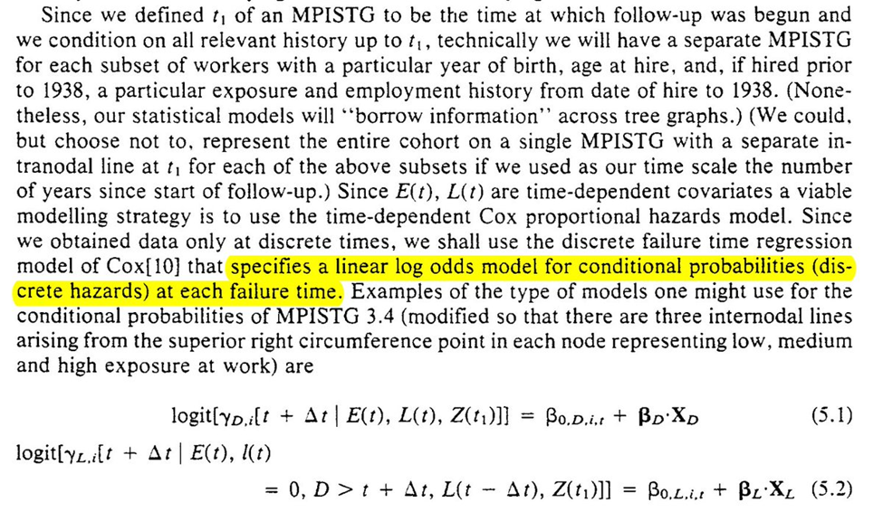
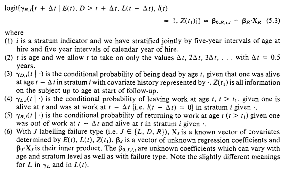
To estimate the parameters for the equations for the g-formula. Robins uses conditional logistic regression for the parameters

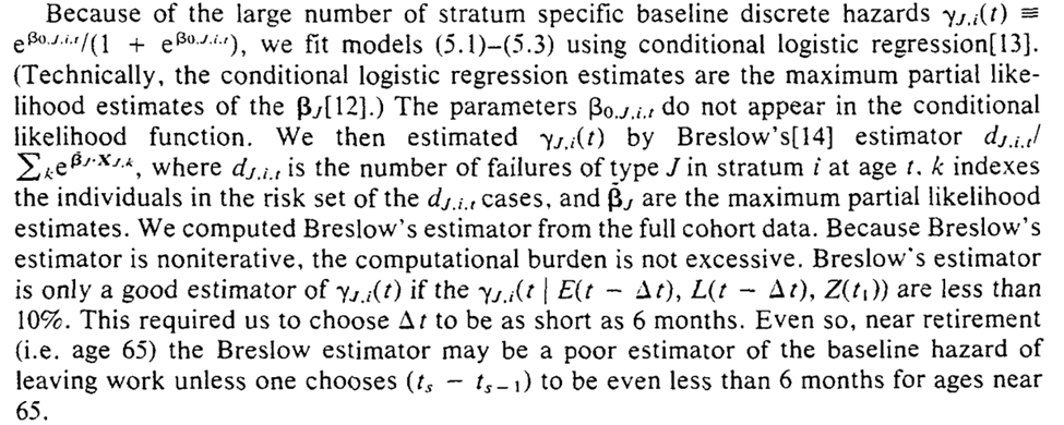
With those estimated parameters, we can then use the Monte Carlo procedure previously described to estimate potential outcomes under the treatment plans of interest

Further mention of our models being correctly specified, and the recommendation to use bootstrapping for inference
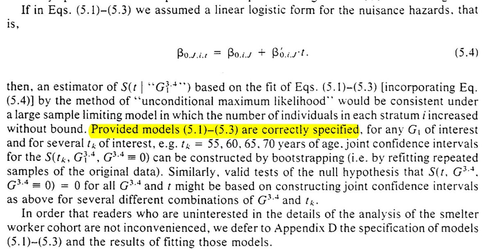
Section 5 closes with further discussion of the issue of parametric model specification. The upside (and teaser for the next section) is that nonparametric null hypothesis testing is possible

6: NONPARAMETRIC TESTS
Section 6 goes through the sharp null hypothesis (that no effect of exposure on any individual). Note that this is weaker than the null of no average effect in the population
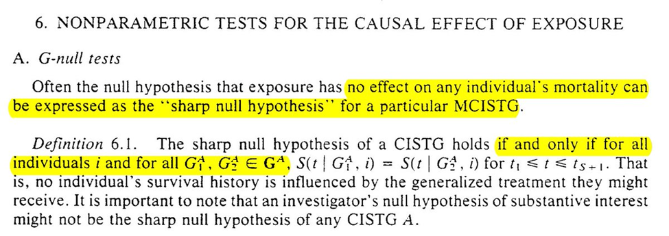
Another way of thinking about this is if there is no individual causal effect (ICE) then there must be no average causal effect (ACE). The reverse (no ACE then no ICE) is not guaranteed.
Robins provides us with the G-null hypothesis as a means of assessing the sharp null (the g-null is that call causal parameters are 0)
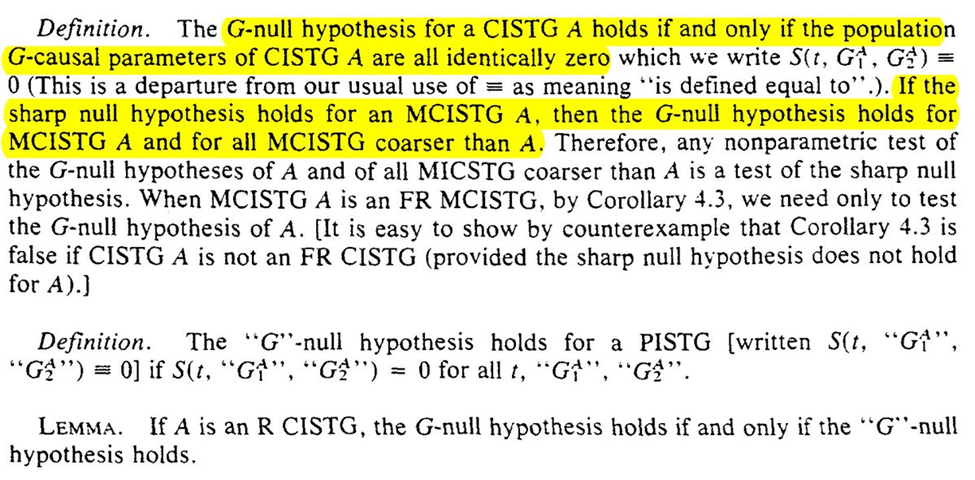
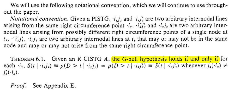

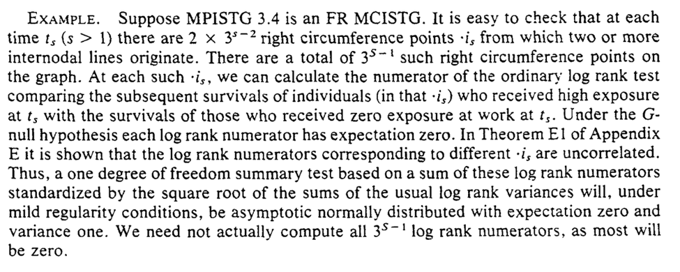
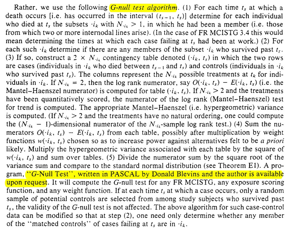
We are given a more complicated procedure for evaluation and a simpler algorithm (the simpler algorithm has PASCAL code which I am curious if anyone still has). Languages that disappear do make me worry a bit about my own work though…
Then we are given some warnings about sparse data. Sparsity can occur through the exposure levels ($A = {0, 1, 2, … a}$) or in follow-up time ($t={0, 1, 2, …\tau}$)
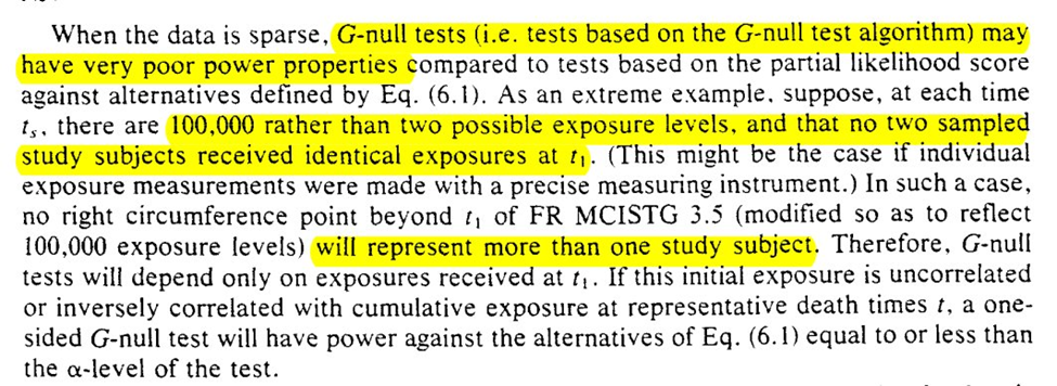
However, not all G-null’s were made the same. When models are introduced for the nuisance functions we can run into problems. Specifically, we can fail to reject at the nominal rate

We are given a list of potential solutions to address the power issue.
We are now given the problem of defining time zero (particularly for the G-null). The more epidemiology I have learned, the more I realize how difficult (and important) defining time zero can be for observational studies (ed: this remains true).
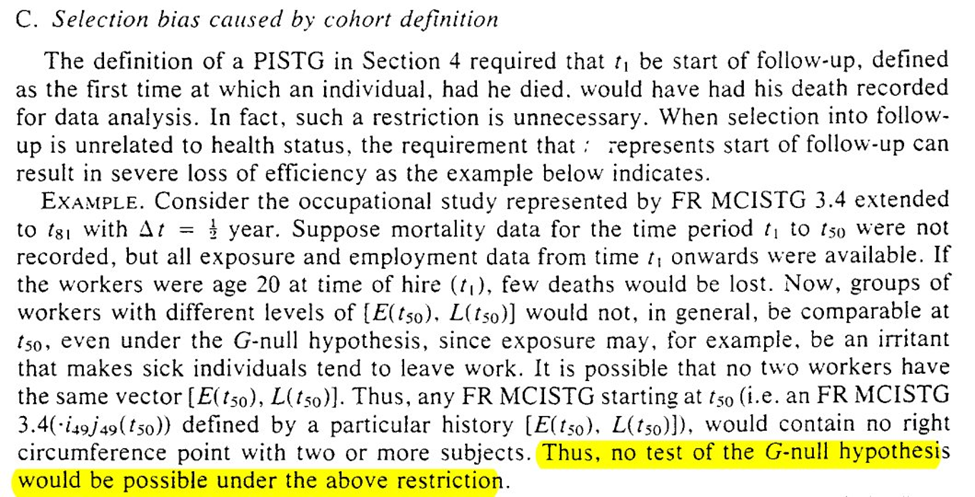
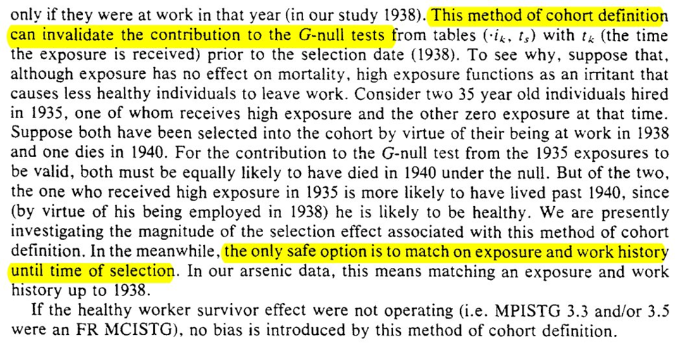
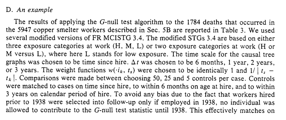
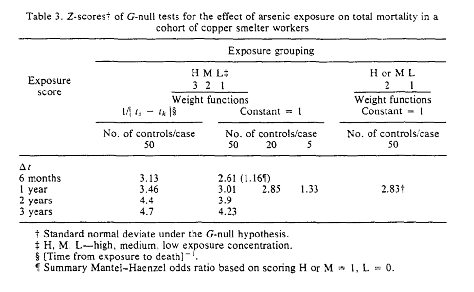
Section 6 concludes with the applied example for the G-null hypothesis. I think Robins’ points about assumptions being slightly wrong and that large sample sizes will reject with near certainty are important
7: MORE ASSUMPTIONS
Section 7 adds some additional a priori assumptions that can allow us to estimate in the context where we don’t have all necessary confounders.
We have the beautifully named: “A-complete Stage 0 PL-sufficient reduced graph of R CISTG A”
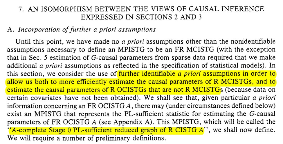
We start with some rules for reducing graph $G_A$ to a counterpart $G_B$. Honestly the language in this section isn’t clear to me despite reading it several times…
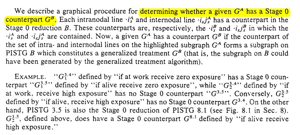
I do think the graphs help a bit though. To me it seems we are narrowing the space of the problem. We are going from multiple divisions at $t_1$ and $t_2$ to only considering the divisions at $t_2$ for a single branch. The reduced STG is a single branch
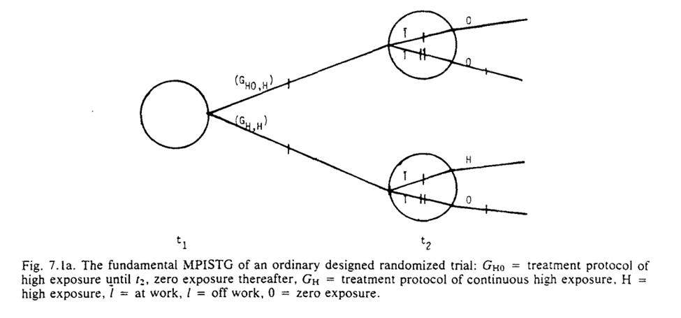

The purpose of our graph reduction is that $G_A$ is identifiable given $G_B$ and the listed assumption $R$
So we can think about G_B as either everyone being set to the same value at $t_1$ OR everyone was off their assigned protocol (and then returned to it at $t_2$)
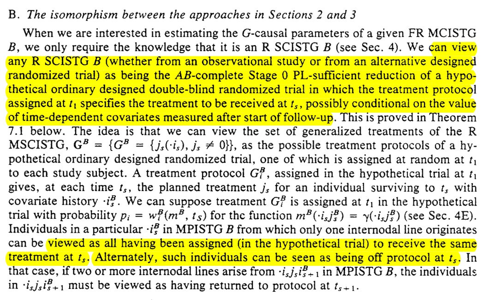
The section ends with the note that we can see if the observed $G_B$ is compatible with a proposed randomization scheme. Section 8 goes on to discuss this and when standard analyses (ignoring time-vary confounding) are valid.
8: WHEN CAN I IGNORE THE METHODOLOGISTS
Section 8 discusses when standard analytic approaches are fine (aka time-varying confounding isn’t as issue for us). Keeping with the occupation theme, it is presented in the context of when employment history can be ignored.
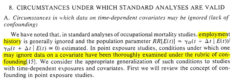
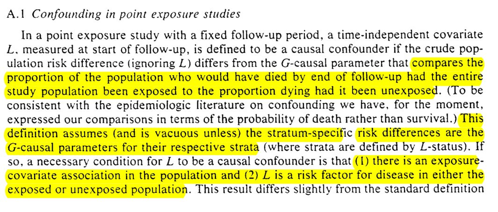
First we go through the simpler case of point-exposures (ie only treatment assignment at baseline matters). Note that while we get something similar to the modern definition, I don’t think the differentiation from colliders is quite there yet (in the language)

Generalization of the point-exposure definition of confounding to time-varying exposures isn’t direct
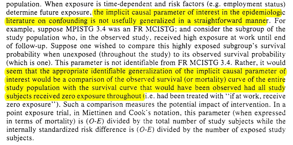
To generalize confounding to time-varying settings, Robins first sets up the conditions for $L$ to be a predictor of the outcome and exposure (at baseline and varying exposures over time)
Again, I think tools like DAG/SWIG are a massive improvement (or an enhancement) to definitions like this. It clarifies colliders and gives a way to a priori specify the causal model. I think it is preferable than calculating to coefficient between various possible $L$ and $Y$
But back to the main question posed by this section, when can be correctly ignore time-varying confounding. We get two sufficient conditions: (1) $L$ does not predict exposure, (2) $L$ does not predict death

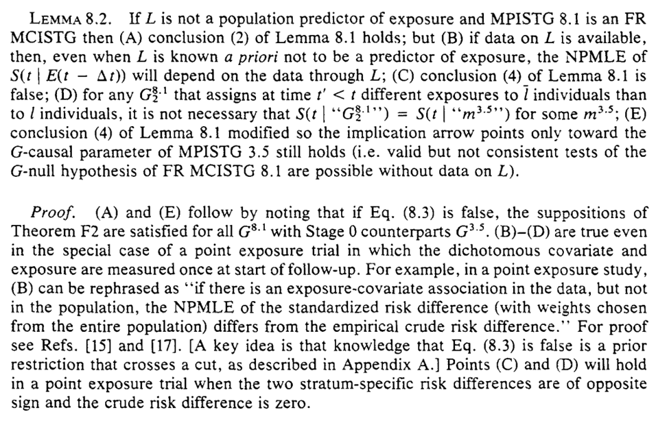
Again, we can easily show this in causal diagrams by lack of an arrow between $L_{t-1} \rightarrow A_{t}$ for the 1st condition or $L_{t-1} \rightarrow Y(t)$ for the 2nd condition. So if there exists no $L$ such that both of the above aren’t true, you can safely ignore me
The next question is when can we ignore the g-methods and use standard approaches for adjustment of time-varying confounding

This is valid when previous exposure does not predict future $L$ (i.e., $A_{t-1} \not\rightarrow L_{t}$). Another way of phrasing is that $A$ effects $Y$ not through $L$.
That’s great and all, but when can be completely ignore $L$ for the null test? Well now we only need both $L \not\rightarrow A$ and $A_{t-1} \not\rightarrow L_{t}$ when $L$ is predictive of $Y$.
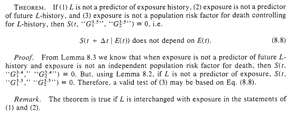
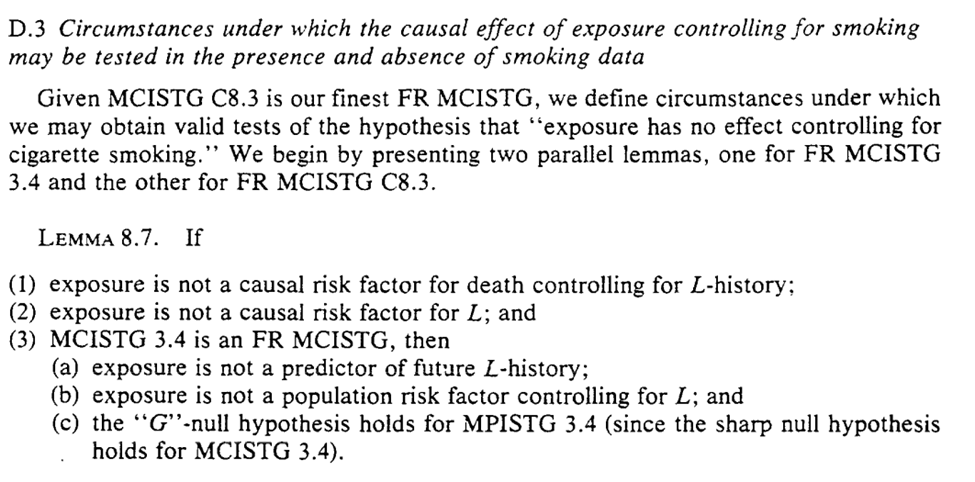
Now that is all a lot of arrows and letters, so Section 8 closes with an example regarding cigarette smoking history. I think it highlights the implausible nature of the previous assumptions that allow you to ignore $L$ (and my methods concerns)

The example provided seems to indicate the difficulty of making any of these assumptions in a defensible way. Robins goes through these in explicit details
Another worthwhile mention from parts I didn’t highlight in this thread: ‘faithfulness’ outside of DAGs

9: CASE-CONTROLS
Back to the irregularly scheduled programming. Honestly, I the more modern methods I have learned, the more confused I have become regarding causal inference from case-control studies. Hopefully I will gain some clarity by the end.
The first part seems to talk about what I wonder (time-varying confounding). The points (particularly the highlights in the last screenshot) seem to be major problems for causal inference with case-controls. However these are when the sampling fractions are unknown

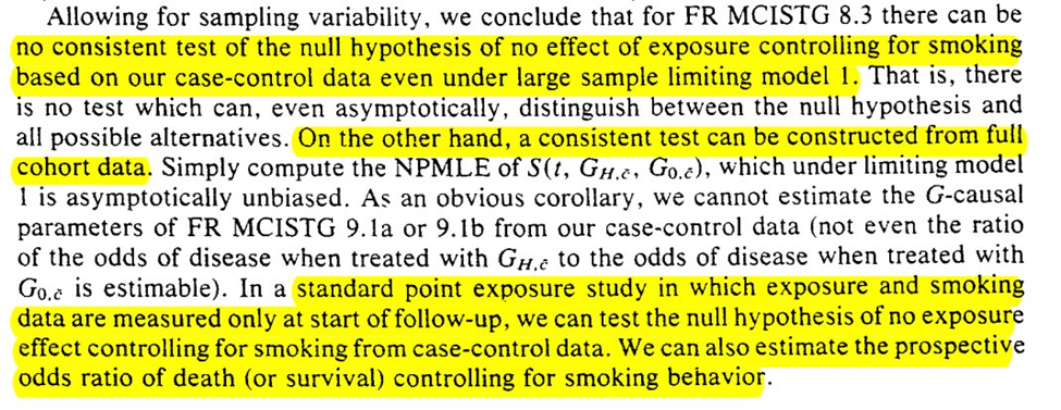
The next example has an interesting result for merging multiple case-control studies. Under this, we can deal with time-varying confounders
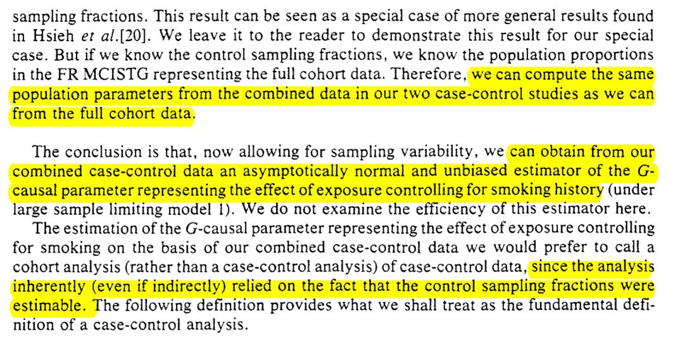
But merging multiple case-control studies doesn’t seem like it can save us. However, the following sentence after example 3 seems to negate that?…
The next subsection starts with an optimistic view that we can construct a nonparam G-null test from case-control. So it looks like I am still missing some pieces in the previous section (let me know if you do because I still don’t follow are re-reading it several times).
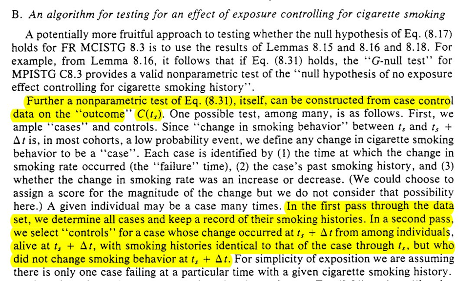
So it looks like we have a hopefully algorithm for causal inference from case-control data in the presence of the healthy-worker effect (time-varying confounding)
However, the title of this subsection seems to indicate my previous statement is too hopefully (I may be getting case-control-induced whiplash). The construction of most case-control studies at the time (and maybe today?) are not designed to work with the proposed algorithm

We get an outline of 3 strategies for selection. Different from the ones I was taught in my programs (since the focus was more on what measure the case-control OR maps to). We also get a secret, bonus 4th strategy
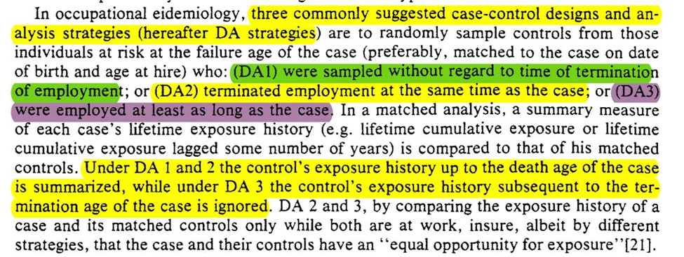
Unfortunately, all 4 of the approaches seem to make (probably) implausible assumptions. The 4th strategy has the weakest, but it still has some problems dealing with time-varying confounding

TLDR: I should read more papers on causal inference and case-control studies (I know there is a chapter in one of the Targeted Learning books, but haven’t gotten to it yet).
10: MODELS AND STUFF WE SAY ABOUT THEM
Section 10 goes through what is termed “artificial healthy worker effect”. The two provided examples focus on it resulting from model misspecification
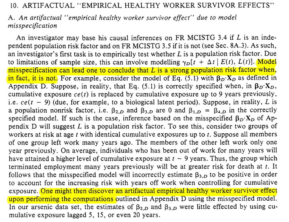
Specifying parametric models is hard. The way I have thought about it lately is to specify the most flexible model as possible and use that. Fill it with as many interaction terms and splines as possible given the data. That way I cover as many possible densities as I can
Avoiding hard constraints on model misspecification also seems to be the main promises of machine learning to me, allow for flexible relationships between the variables that minimizes what I need to specify directly. But there is still lots to do on this front
Check out my paper on cross-fitting with machine learning if you want to read more on using machine learning for estimation (at least I made it to section 10 without any self-promotion). There are also a lot of other great papers referenced there
The next example is what I think is along the lines of measurement error, or coarsening. I use the term coarsening because we have $L =$ {keep working, laid off, quit}, but we only use $L^* =$ {keep working, stop working}

That collapsing is sometimes called coarsening (first I understood the term was in reading Tsiatis’s semiparametric theory book)
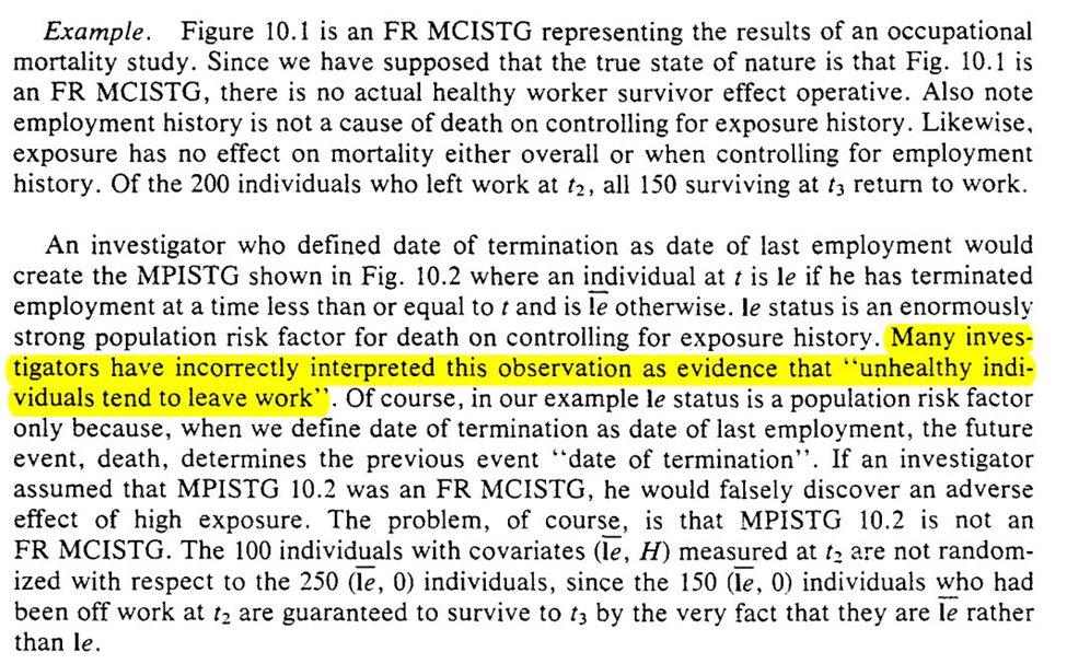
And that is actually it for section 10 (short one I know). Next section is a bit longer and returns to the other proposed approach way back in the beginning. We will see why it doesn’t work
11: CONTROL VIA MIN(LATENT PERIOD)
Happy Halloween! Let’s discuss the spOoOoOoOokiest of things; time-varying confounding.
This is the penultimate section and returns to the approach described in the intro of addressing the healthy worker effect via latent period assumptions
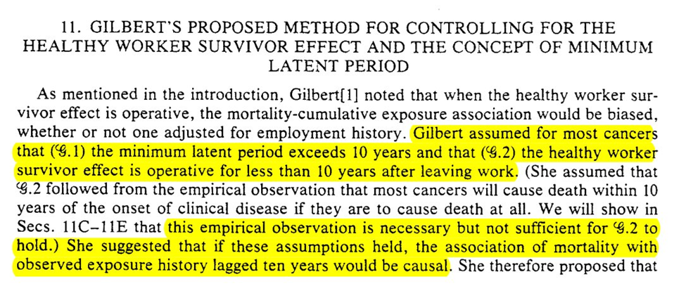
It looks like the quantity estimated is a causal parameter under a certain set of assumptions that we will learn in the following sections. Where (G1) is min(latent) > 10yr, (G2) is healthy worker <10 after leaving work
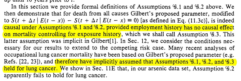
But we also need an additional assumption for the approach to work: (G3) employment history has no effect on $Y$ controlling for exposure history
Going slightly out of order from the paper, Robins goes through (G1). A first version that stipulates no time-varying confounding is presented, but Robins gives us a second that allows for time-varying confounding and proceeds under that scenario
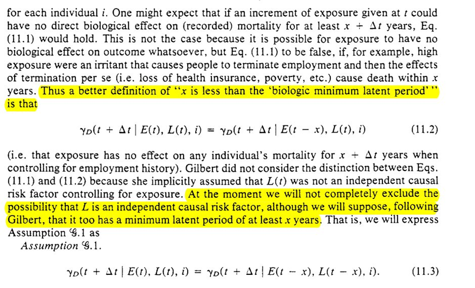
Given some definitions, Robins then presents a very detailed and thorough proof of Lemma 11.1
For (G2), we assume deterministic outcomes, such that there are ‘doomed’ people for $Y$. Then we get the formal definition
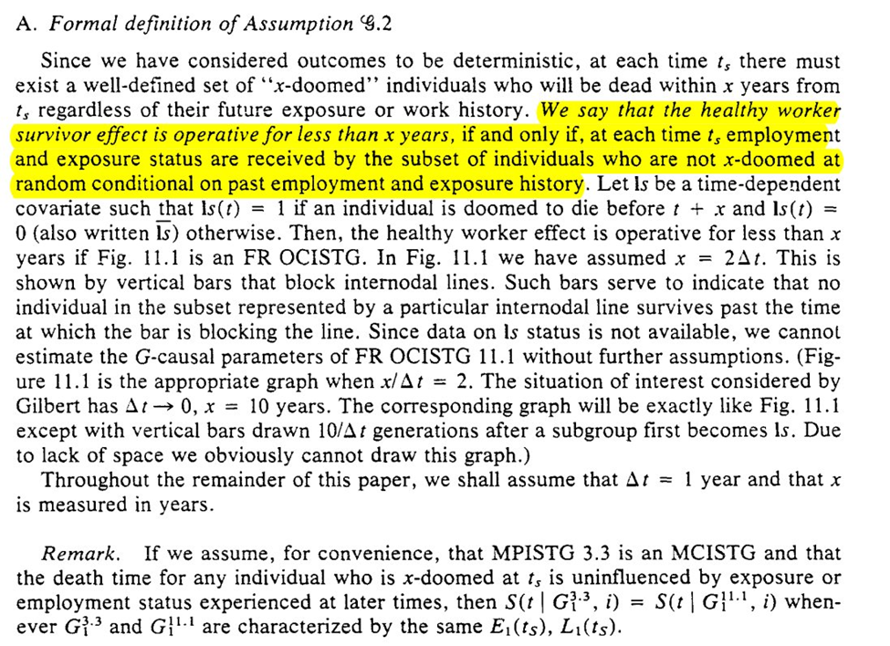
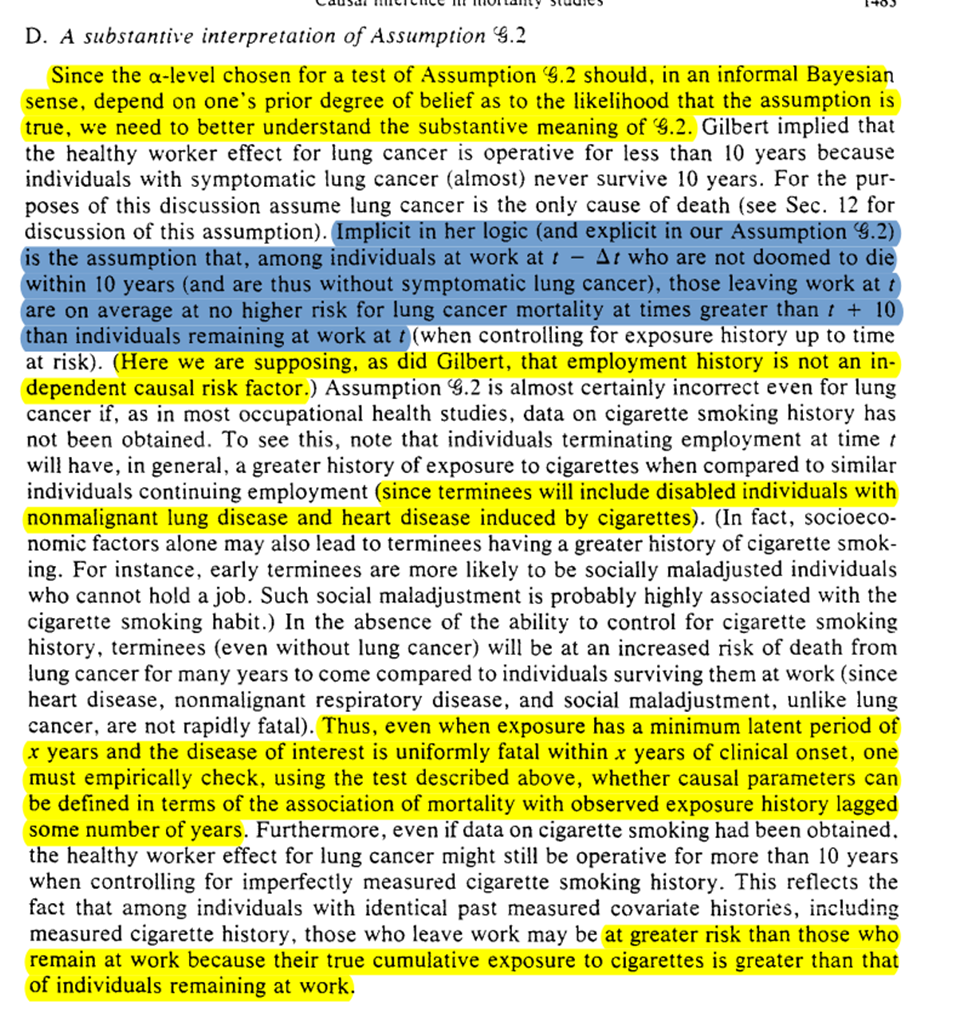
Later on (but I’m putting it here), we get a substantive description of what this means. We are saying $L(t)$ is not related to $Y$ (since we already know $L(t-1) \rightarrow A(t)$). Robins puts this in the context of lung cancer, and then shows the problem of the assumption with smoking ($U$).
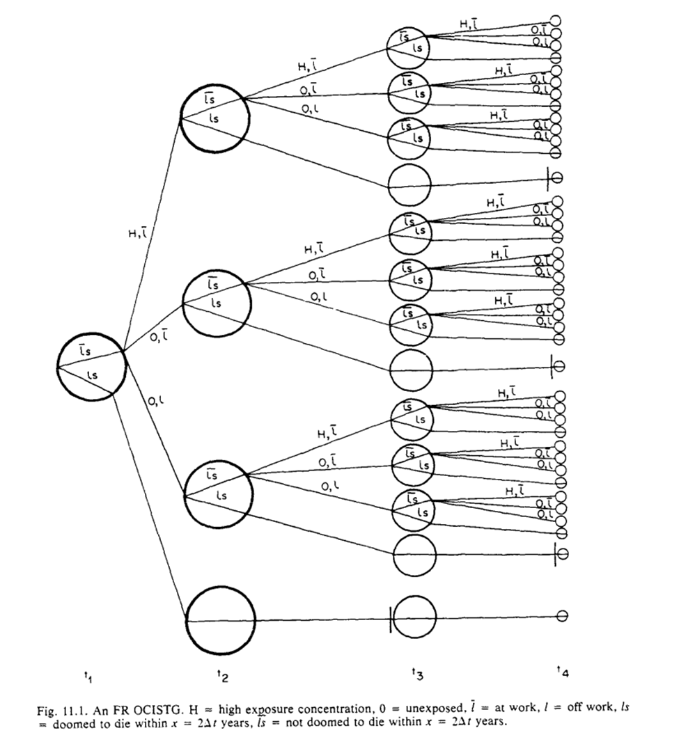
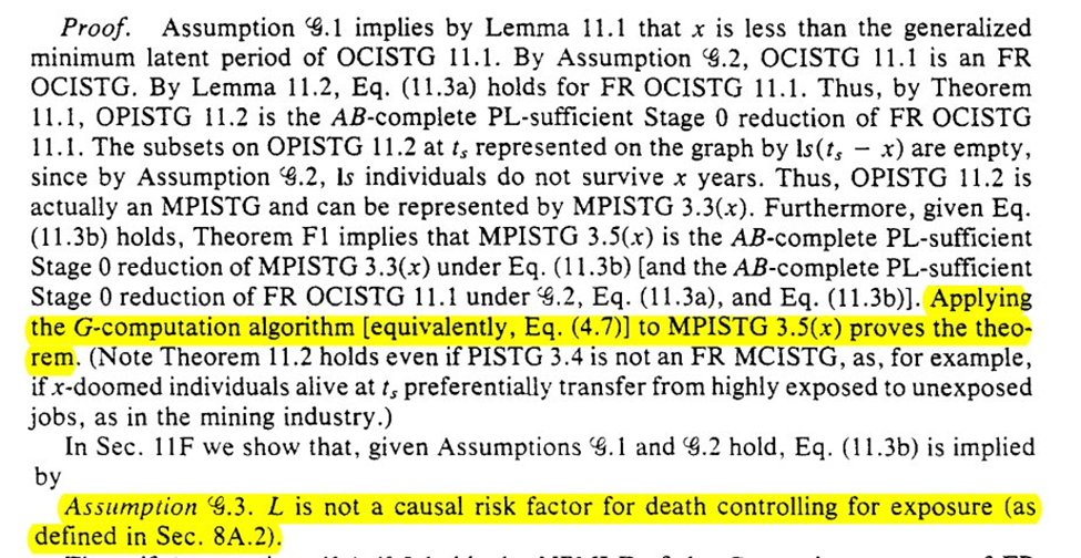
Then Robins draws out the tree graphs under (G1) and (G2). By contrasting Gilbert’s estimand with the causal tree graphs and g-formula, we then get to see why we need to have assumption (G3)
Next we are tasked with the problem of assessing the validity of (G1)-(G3). We can do that by comparing $A=1$ versus $A=0$ at $T=t$, for those with $A=1$ at $T=t-1$. We then get the algorithm for assessing the assumptions

However, the algorithms are probably not going to work well in-practice. Sparsity of data, especially if measured at fine-grained time intervals, may preclude being able to adequately assess. We could use models but then we need to assume our models are correct (unlikely)
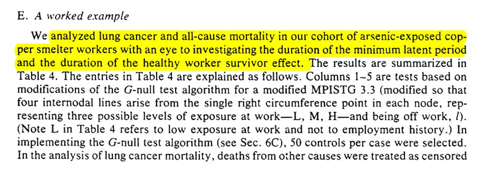
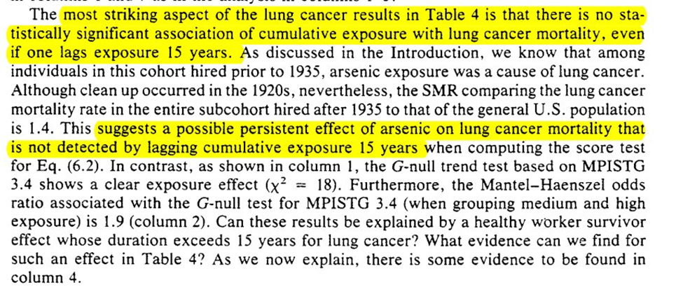
We then get an example using the arsenic -> lung cancer / mortality example. In the example Robins finds that an effect of arsenic on lung cancer can be hidden by using an exposure lag of 15 years
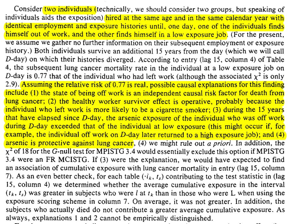
To work through explanations for the observations we are given a case of 2 individuals and 4 explanations for the divergence. 3rd and 4th are ruled out, which leaves us with off-work is a time-varying confounder OR healthy worker effect
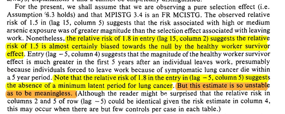
So then we assume that it is a result of only explanation 2. Based on this, Robins states there is evidence of the healthy worker effect persisting (but that he doesn’t believe it to be the full story for the divergence)
That concludes Section 11. Next time is Section 12, which is the grand finale
12: EVERYTHING ENDS
We are at the end friends. The last section of Robins 1986.
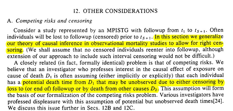
We start with censoring and competing risks. I don’t like how this section starts since it seems to imply we can handle those issues in the same way
If we treat competing risks as ‘censoring’, we are estimating the effect in a world where we can prevent all competing events…
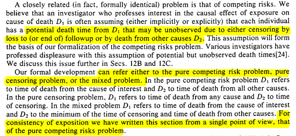
Robins does give us this weird world we are estimating when we treat competing risks as censored

However, you don’t have to make this estimand. You can do the parametric g-formula machinery with two outcome models (one for competing risk, one for outcome). Simulate under the intervention. Then analyze that simulated data using an appropriate estimator (e.g. Aalen-Johansen)
Next is what we can learn with and without data on cigarette smoking. Again we are in a ‘world’ where only lung cancer deaths occur.
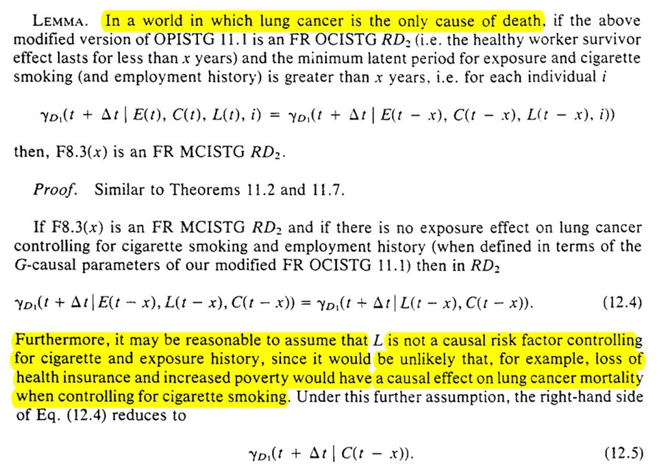
Unfortunately, there isn’t much to do in the setting of competing risks when you have an unobserved confounder for both types of outcomes. This holds true for estimation

We can do some hypothesis testing though. However, we can’t make progress with confounding (particularly time-varying confounding which is likely in the example)
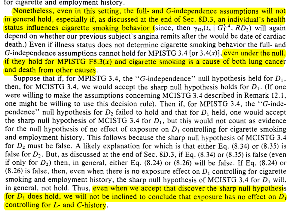
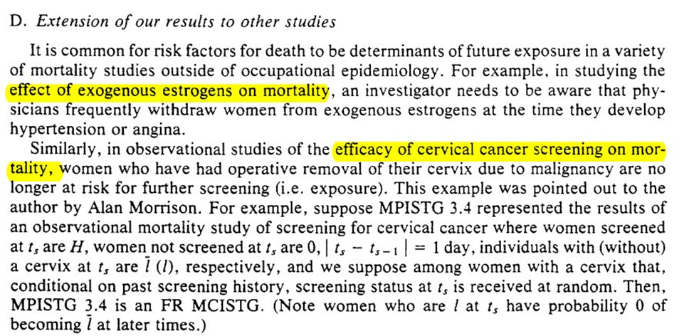
The final subsection is extension to other studies. The results can be extended to many other studies where time-varying confounding can occur. Robins provides several examples outside of occupational health research
If you’ve made it this far and want some additional g-formula papers, here are some suggestions on what to read next
That concludes Robins 1986 (aside from the Appendix, but that’s more of a Scouring of the Shire anyways)